Read my latest on Saudi’s views toward the Iran War in The Conversation.
When Using OLS Hurts
Re-examining the Relationship Between Tenure Denial and Race in Masters-Waage et al. (2024)
People often use OLS for bounded continuous variables even though we know it isn’t the correct model. Ordered beta regression is a better model–but hard to predict when the results will change. For the article discussed in this blog post, OLS hid an important empirical relationship in the data.
R
Statistics
Ordered Beta Regression
Tenure
Race
Author
Robert Kubinec
Published
May 14, 2026
Ordinary least squares–also commonly called regression–is the dominant model in the social sciences. I’m sure it always will be. But there are times and places where this workhorse fails to deliver a useful answer to a research question. I developed ordered beta regression for one of these cases: bounded continuous outcomes, also called proportions. Proportions arise quite often in the social and biological sciences. There are two common sources of this kind of data:
We are measuring a continuous outcome that we want to standardize for comparability (i.e., measure it relative to a total).
We are using a measurement device like a slider that has physical bounds (such as the oft-used feeling thermometer/visual analog scale).
For this post, I will examine an empirical paper that had an outcome meeting the first condition. Masters-Waage et al. (2024) analyzed tenure decisions from a consortium of five major research universities, amounting to over a thousand tenure votes at the department and college level. Measuring this outcome as a proportion comes naturally by dividing the total votes by the size of the voting members (i.e. the department or collegiate tenure committee). In fact, it is so natural that it might not even have occurred to you that it could be modeled differently, but it would be possible to also model the raw number of votes with the Poisson or Negative Binomial distributions.
Alternatively, we could model the total vote numbers with the Binomial distribution, though in this case that might be unwise as the Binomial model will put more weight on votes with a higher total of voting members. For tenure, though, the collegiate committee may be smaller in size than the department tenure vote, so we want to standardize that issue away by simply using the proportion who voted for a candidate.
Probably more information than you wanted to think about, but hey, I’m an academic. It’s literally my job to think too much.
Masters-Waage et al. (2024) use OLS for all of their tenure proportion outcomes. I don’t fault them for it; my R package ordbetareg did not appear until they had largely completed their research. Indeed, my aim is not to “take on” anyone; rather, I want to show a concrete example where effects that were reported as non-significant by OLS in fact become more precise and meaningful with ordered beta regression.
Why Ordered Beta?
The ordered beta regression model is admittedly more complicated than OLS and requires more computational oomph. At the same time, with modern computers and software packages, the difference is fairly trivial, especially with a dataset of 1,000 cases. But OLS is a tough competitor–the model does a great job with the conditional mean of the distribution. The problem is that OLS is based on the Normal distribution, i.e. the classic bell-curve shape, which is uni-modal and symmetric. As a consequence, OLS cannot respect boundaries such as a lower limit of 0% and 100% of tenure votes. To OLS, each number is the same as another number, which is why it is considered the classic linear model. Pure linearity works well in many cases–just not all cases.
Indeed, it’s possible to use OLS and have it return a very similar estimate to ordered beta regression even though OLS isn’t made for proportions. But the difference can be significant, and importantly, it’s very unwise to choose a model based on the results you get. Given issues with researcher discretion (the so-called garden of forking paths), you should always choose the best model for your research design. That way, if the results don’t go way (or they do), you can defend your results regardless.
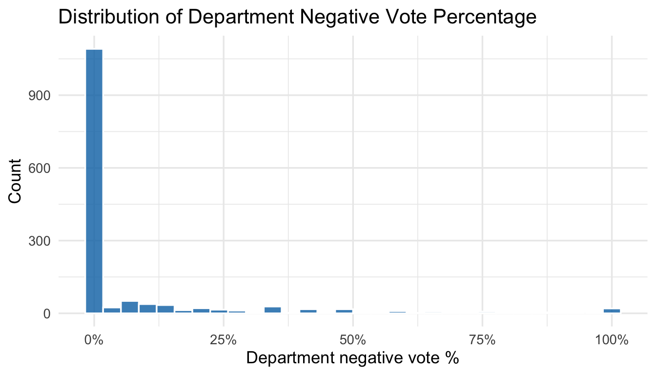
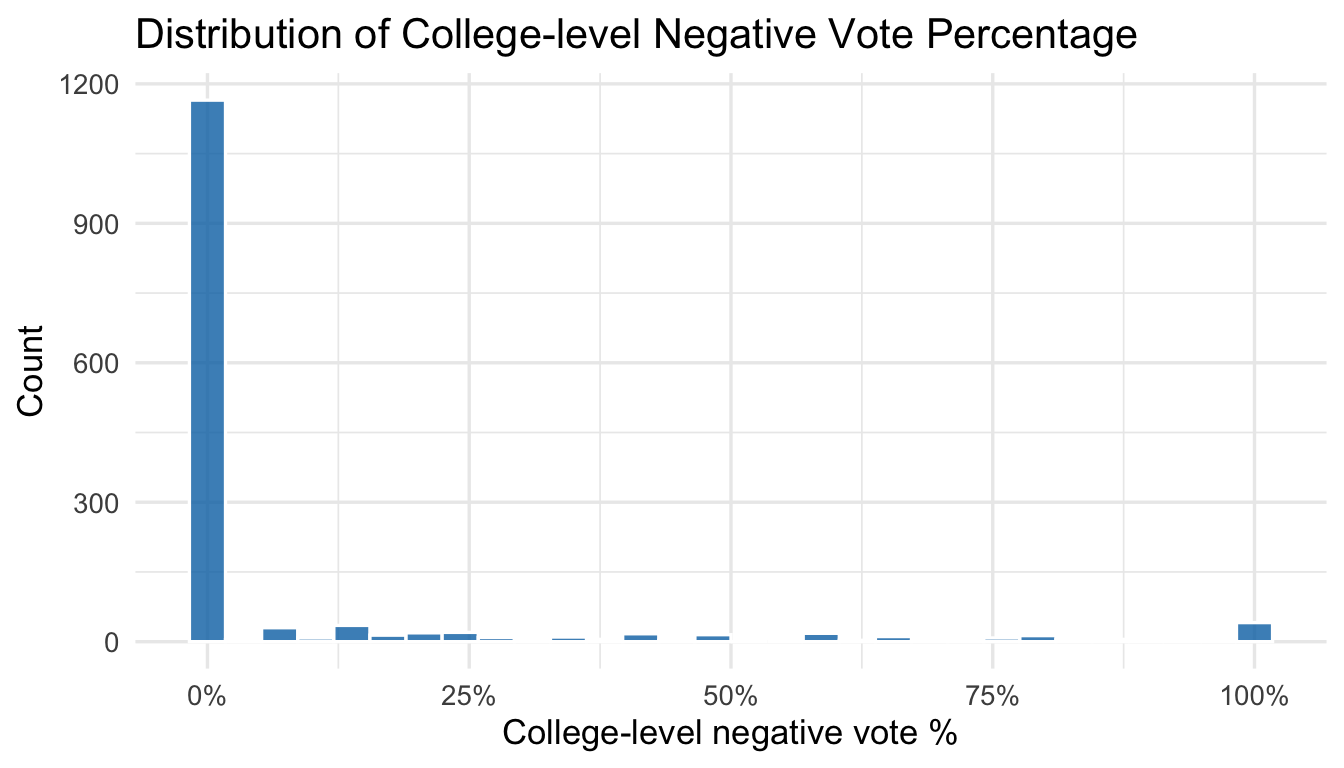
For the Masters-Waage et al. (2024) study, the issue of non-linearity arises because there are a lot of tenure votes that are unanimous. Academics tend to like people in their own department, and oftentimes people who aren’t doing well in the tenure track will withdraw before submitting their files. As a consequence, split votes are relatively rare. The histograms below show what these distributions look like for department-level and college-level tenure votes:
Show the code
ggplot(candidates, aes(x = department_negative_vote_percentage)) +geom_histogram(bins =30, fill ="#0072B2", color ="white", alpha =0.8) +scale_x_continuous(labels = scales::percent_format()) +labs(title ="Distribution of Department Negative Vote Percentage",x ="Department negative vote %",y ="Count" ) +theme_minimal(base_size =13)
Show the code
ggplot(candidates, aes(x = college_committee_negative_vote_percentage)) +geom_histogram(bins =30, fill ="#0072B2", color ="white", alpha =0.8) +scale_x_continuous(labels = scales::percent_format()) +labs(title ="Distribution of College-level Negative Vote Percentage",x ="College-level negative vote %",y ="Count" ) +theme_minimal(base_size =13)
The authors reversed the scale so that 0% means everyone voted for the candidate. As can be seen, for both departments and college-level votes, most votes are unanimous. Unfortunately, while OLS can still model the average of this distribution, the variance (error term) will be way off. An OLS model will likely predict that the department negative vote is below 0%, which of course is nonsense.
Replication
In this section, I replicate some of the main findings in the paper for the proportion of department-level negative votes on tenure, comparing OLS to ordered beta regression side-by-side. The main research question in this paper is fascinating and important: are minority faculty disadvantaged in tenure decisions? The authors account for differences in faculty productivity (the h-index) and, intriguingly, the general tone of external letters. At the end of this blog post, I also look at the college-level outcomes.
My main goal here is not to evaluate the research design, but it is important to note that it is very difficult to infer causality with observational data when the outcome is tenure. There are lots of factors that differ across racial groups, fields, and as I noted earlier, lots of strategic behavior where people withdraw their cases if the outcome doesn’t look good. Given those caveats, though, this study has some excellent data and the authors should be commended for making it very easy to replicate their findings. That’s how science improves! 🙌
Main Findings: Are Minority Faculty Disadvantaged in Promotion and Tenure Decisions?
I’ll first reproduce their unadjusted model that examines whether what they call under-represented minority (URM) status, a binary indicator, is associated with higher or lower negative department vote proportions for all promortions (i.e., promotion to associate professor or full professor, Model 1 in Table 1 in their paper) along with the ordered beta regression version. To make the ordered beta regression estimates comparable to the OLS estimates, I’ll use the avg_slopes function in the marginal_effects package to get estimates in the scale of the outcome, i.e., as a fraction of department vote:
Running MCMC with 2 sequential chains...

Chain 1 finished in 3.1 seconds.
Chain 2 finished in 3.2 seconds.

Both chains finished successfully.
Mean chain execution time: 3.1 seconds.
Total execution time: 6.5 seconds.
Show the code
avg_ord1 <-avg_slopes(ord1)
Show the code
# make a nice table with modelsummary and relabel everythingms_compare(lm1, avg_ord1, "URM → dept. negative vote % — no controls, full sample")
URM → dept. negative vote % — no controls, full sample
LM (original)
Ordbetareg (new)
Outcome: proportion of votes [0, 1]. Coefficients equal changes in proportions.
95% frequentist CI (R lm) and 95% posterior CrI (Ordbetareg) shown.
URM candidate
0.030
0.038
[-0.005, 0.065]
[0.004, 0.076]
Num.Obs.
1422
1422
As can be seen, the OLS (LM) model shows an association between URM status and negative tenure votes that is 22.2% smaller than the size of the ordered beta regression model. OLS shows that URM candidates receive 3% more negative votes while ordered beta regression shows that URM candidates receive 3.8% more votes. This is an unadjusted, straightforward comparison with a binary covariate, so it is a particularly notable difference considering that both models are quite similar in form (i.e., neither is a fancy ML-style model). What is likely happening is that OLS is pulling the differences toward the mode at 0, while ordered beta regression is taking into account differences in the full distribution, including the small but quite important votes where all faculty voted against a candidate (!!). Again, very few if any statisticians will argue that OLS is the right model for a distribution like the one show above… so this is an easy win! 🙌
Sure, 22.2% isn’t earth-shattering–but remember, all we are doing here is switching the statistical distribution for the outcome. This improvement is free, in other words–and rests on a better statistical foundation regardless. If it didn’t, we might consider this a form of \(p\)-hacking, but one of the best ways to avoid the temptation to \(p\)-hack is to start with the best model for the outcome.
I also want to give some props to the authors again for releasing their data and code and for reporting “null” results (the OLS estimate is not significant at conventional levels). If they hadn’t done that, I might have never run the data with ordered beta and discovered this fairly noticeable discrepancy.
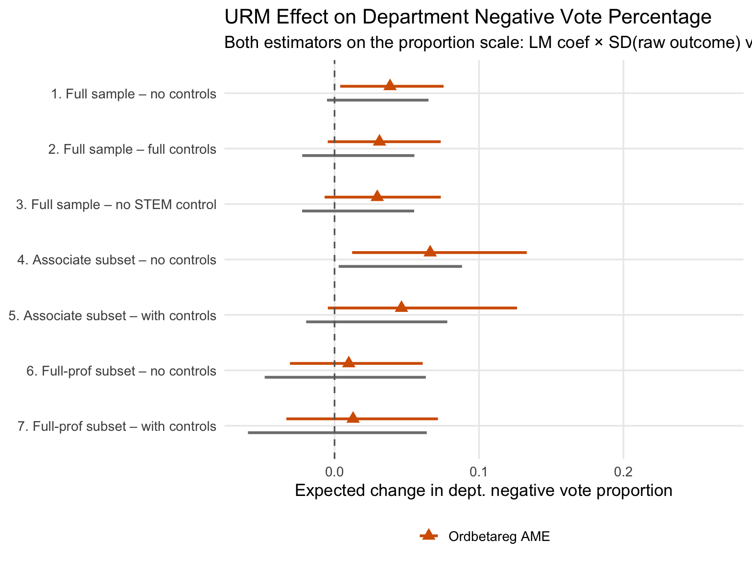
The authors fit quite a large number of further models with a variety of adjustments with covariates. I won’t walk through all of them but rather summarize them in a plot showing OLS vs. ordered beta regression estimates. These include models that subset by whether the department votes on promotion to associate or full professor.
The code block shows the details for all the models run:
Running MCMC with 2 sequential chains...

Chain 1 finished in 10.2 seconds.
Chain 2 finished in 10.1 seconds.

Both chains finished successfully.
Mean chain execution time: 10.2 seconds.
Total execution time: 20.6 seconds.
Show the code
# Average marginal effects for candidate_urm_num from each ordbetareg model.# These are on the proportion scale (same units as the raw outcome), making# them directly comparable to LM coefficients back-transformed by × SD.ame1 <-avg_slopes(ord1, variables ="candidate_urm_num")ame2 <-avg_slopes(ord2, variables ="candidate_urm_num")ame3 <-avg_slopes(ord3, variables ="candidate_urm_num")ame4 <-avg_slopes(ord4, variables ="candidate_urm_num")ame5 <-avg_slopes(ord5, variables ="candidate_urm_num")ame6 <-avg_slopes(ord6, variables ="candidate_urm_num")ame7 <-avg_slopes(ord7, variables ="candidate_urm_num")
and below is the marginal effects plot:
Show the code
extract_urm <-function(lm_mod, ame_df, label) { lm_row <-coef(summary(lm_mod))["candidate_urm_num", ] ame_row <- ame_df[ame_df$term =="candidate_urm_num", ]tibble(analysis = label,lm_est = lm_row[["Estimate"]],lm_lo = (lm_row[["Estimate"]] -1.96* lm_row[["Std. Error"]]),lm_hi = (lm_row[["Estimate"]] +1.96* lm_row[["Std. Error"]]),lm_p = lm_row[["Pr(>|t|)"]],ame_est = ame_row$estimate,ame_lo = ame_row$conf.low,ame_hi = ame_row$conf.high,lm_sig = lm_row[["Pr(>|t|)"]] <0.05,ame_sig = ame_row$conf.low >0| ame_row$conf.high <0,same_sign =sign(lm_row[["Estimate"]]) ==sign(ame_row$estimate) )}results <-bind_rows(extract_urm(lm1, ame1, "1. Full sample – no controls"),extract_urm(lm2, ame2, "2. Full sample – full controls"),extract_urm(lm3, ame3, "3. Full sample – no STEM control"),extract_urm(lm4, ame4, "4. Associate subset – no controls"),extract_urm(lm5, ame5, "5. Associate subset – with controls"),extract_urm(lm6, ame6, "6. Full-prof subset – no controls"),extract_urm(lm7, ame7, "7. Full-prof subset – with controls"))# Long format: one row per model × estimatorplot_data <-bind_rows( results |>transmute( analysis,estimator ="OLS",est = lm_est, lo = lm_lo, hi = lm_hi,sig = lm_sig ), results |>transmute( analysis,estimator ="Ordbetareg AME",est = ame_est, lo = ame_lo, hi = ame_hi,sig = ame_sig )) |>mutate(analysis =fct_rev(factor(analysis)),estimator =factor(estimator, levels =c("OLS", "Ordbetareg AME")) )ggplot(plot_data,aes(x = est, xmin = lo, xmax = hi, y = analysis,color = estimator, shape = estimator)) +geom_pointrange(position =position_dodge(width =0.5),size =0.7, linewidth =1 ) +geom_vline(xintercept =0, linetype ="dashed", color ="grey40") +scale_color_manual(values =c("OLS"="#0072B2","Ordbetareg AME"="#D55E00")) +scale_shape_manual(values =c("OLS"=16,"Ordbetareg AME"=17)) +labs(title ="URM Effect on Department Negative Vote Percentage",subtitle ="Both estimators on the proportion scale",x ="Expected change in negative vote proportion",y =NULL,color =NULL, shape =NULL ) +theme_minimal(base_size =13) +theme(legend.position ="bottom",panel.grid.minor =element_blank() )
The ordered beta regression estimate of URM status isn’t always statistically significant at the 5% - 95% level (to the extent that comparison works with a Bayesian model), but the coefficient is always bigger, sometimes by a larger fraction than for the unadjusted model. I take this as additional support for the authors’ findings; given the limited size of the dataset, it isn’t surprising that the models with controls are a bit less powered, and the coefficients remain large. For sure, having more power would be more helpful, but collecting this type of data is hard. I think we can safely conclude here that URM status has an association with more negative department tenure votes even if there is residual uncertainty–which probably requires more data collection to provide additional confirmation.
To conclude, this seems like a situation where ordered beta regression is the preferred model. However, to be a valid research practice, ordered beta regression should be preferred because it is a better model, not just because it gives results in the authors’ expected direction. By making ordered beta regression the default specification, rather than OLS, scholars can get better, usually more precise estimates, while also employing a model that has clear statistical foundations.
Extending the Analysis to College-Level Votes
In this section, I’ll repeat the same analysis (switching out OLS for ordbetareg), but the outcome is now college_committee_negative_vote_percentage, that is, how do the college-level committees vote on URM candidate tenure files? As noted above, these distributions are also highly skewed and contain a significant share of zeroes (unanimous votes).
Running MCMC with 2 sequential chains...

Chain 1 finished in 5.6 seconds.
Chain 2 finished in 6.0 seconds.

Both chains finished successfully.
Mean chain execution time: 5.8 seconds.
Total execution time: 11.8 seconds.
Show the code
avg_cord1 <-avg_slopes(cord1)
Show the code
ms_compare(clm1, avg_cord1, "URM → college negative vote % — no controls, full sample")
URM → college negative vote % — no controls, full sample
LM (original)
Ordbetareg (new)
Outcome: proportion of votes [0, 1]. Coefficients equal changes in proportions.
95% frequentist CI (R lm) and 95% posterior CrI (Ordbetareg) shown.
URM candidate
0.077
0.069
[0.035, 0.118]
[0.028, 0.118]
Num.Obs.
1457
1457
What the table above shows is that with these outcomes, the ordbetareg model is slightly smaller the OLS: estimate of the URM effect is -11.8% smaller. OLS implies URM candidates receive 7.7% more negative college votes, while ordered beta regression puts that figure at 6.9%.
These results show that (of course) ordbetareg does not always inflate OLS results. If it did, there would be something very wrong with the distribution (i.e., it would be equal to OLS plus some constant). Why the estimate is slightly deflated can be difficult to determine, but again, this only serves to highlight how the model should be chosen for principled reasons, not because it gives a favored or dis-favored outcome.
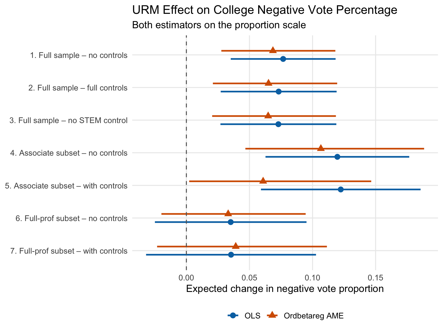
In the plot below I compare OLS and ordbetareg for the full range of college-level outcome votes:
Running MCMC with 2 sequential chains...

Chain 1 finished in 16.2 seconds.
Chain 2 finished in 17.3 seconds.

Both chains finished successfully.
Mean chain execution time: 16.8 seconds.
Total execution time: 33.7 seconds.
Show the code
# Average marginal effects for candidate_urm_num from each college-level model,# on the proportion scale so they are comparable to the LM coefficients.came1 <-avg_slopes(cord1, variables ="candidate_urm_num")came2 <-avg_slopes(cord2, variables ="candidate_urm_num")came3 <-avg_slopes(cord3, variables ="candidate_urm_num")came4 <-avg_slopes(cord4, variables ="candidate_urm_num")came5 <-avg_slopes(cord5, variables ="candidate_urm_num")came6 <-avg_slopes(cord6, variables ="candidate_urm_num")came7 <-avg_slopes(cord7, variables ="candidate_urm_num")
Show the code
college_results <-bind_rows(extract_urm(clm1, came1, "1. Full sample – no controls"),extract_urm(clm2, came2, "2. Full sample – full controls"),extract_urm(clm3, came3, "3. Full sample – no STEM control"),extract_urm(clm4, came4, "4. Associate subset – no controls"),extract_urm(clm5, came5, "5. Associate subset – with controls"),extract_urm(clm6, came6, "6. Full-prof subset – no controls"),extract_urm(clm7, came7, "7. Full-prof subset – with controls"))college_plot_data <-bind_rows( college_results |>transmute( analysis,estimator ="OLS",est = lm_est, lo = lm_lo, hi = lm_hi,sig = lm_sig ), college_results |>transmute( analysis,estimator ="Ordbetareg AME",est = ame_est, lo = ame_lo, hi = ame_hi,sig = ame_sig )) |>mutate(analysis =fct_rev(factor(analysis)),estimator =factor(estimator, levels =c("OLS", "Ordbetareg AME")) )ggplot(college_plot_data,aes(x = est, xmin = lo, xmax = hi, y = analysis,color = estimator, shape = estimator)) +geom_pointrange(position =position_dodge(width =0.5),size =0.7, linewidth =1 ) +geom_vline(xintercept =0, linetype ="dashed", color ="grey40") +scale_color_manual(values =c("OLS"="#0072B2","Ordbetareg AME"="#D55E00")) +scale_shape_manual(values =c("OLS"=16,"Ordbetareg AME"=17)) +labs(title ="URM Effect on College Negative Vote Percentage",subtitle ="Both estimators on the proportion scale",x ="Expected change in negative vote proportion",y =NULL,color =NULL, shape =NULL ) +theme_minimal(base_size =13) +theme(legend.position ="bottom",panel.grid.minor =element_blank() )
Again, most of the ordbetareg models are slightly deflated relative to OLS. That may be confusing given that the department-level votes were inflated, but it’s important to note that these are two different statistical distributions. There is no easy 1:1 correspondence between them.
It is important to flag the one big outlier, which is the associate professor model with controls in the figure above. In this case, the ordbetareg estimate is much smaller than OLS. Why did this discrepancy occur? Adding controls to a model can sharpen the disagreements between models because it induces correlation in the conditional average (expectation). The histograms that are plotted above show skewness for the distribution as a whole, but subsets of the population, such as associate professors with high productivity, could have far sharper non-linearities. As a consequence, statistical distributions can have outsize impacts as the model specification becomes more complex–and again, this is yet another reason to start with a statistical distribution you have some confidence in.
Summary
OLS can buy you a lot of things… but not happiness. Only ordered beta can do that. 😎
References
Masters-Waage, Theodore, Christiane Spitzmueller, Ebenezer Edema-Sillo, et al. 2024. “Underrepresented Minority Faculty in the USA Face a Double Standard in Promotion and Tenure Decisions.”Nature Human Behaviour 8 (11): 2107–18. https://doi.org/10.1038/s41562-024-01977-7.