# ── Helper: extract URM row from each model pair ───────────────────────────
extract_urm <- function(lm_mod, ord_mod, label, lm_sd) {
# LM
lm_row <- coef(summary(lm_mod))["candidate_urm_num", ]
# Ordbetareg: fixef() from brms returns Estimate, Est.Error, Q2.5, Q97.5
ord_row <- fixef(ord_mod)["candidate_urm_num", ]
# Posterior probability > 0
draws <- as_draws_df(ord_mod)[["b_candidate_urm_num"]]
pp_pos <- round(mean(draws > 0), 3)
tibble(
analysis = label,
lm_est = lm_row[["Estimate"]],
lm_lo = lm_row[["Estimate"]] - 1.96 * lm_row[["Std. Error"]],
lm_hi = lm_row[["Estimate"]] + 1.96 * lm_row[["Std. Error"]],
lm_p = lm_row[["Pr(>|t|)"]],
lm_est_prop = lm_row[["Estimate"]] * lm_sd,
lm_lo_prop = (lm_row[["Estimate"]] - 1.96 * lm_row[["Std. Error"]]) * lm_sd,
lm_hi_prop = (lm_row[["Estimate"]] + 1.96 * lm_row[["Std. Error"]]) * lm_sd,
ord_est = ord_row[["Estimate"]],
ord_lo = ord_row[["Q2.5"]],
ord_hi = ord_row[["Q97.5"]],
pp_pos = pp_pos,
same_sign = sign(lm_row[["Estimate"]]) == sign(ord_row[["Estimate"]]),
lm_sig = lm_row[["Pr(>|t|)"]] < 0.05,
ord_sig = ord_row[["Q2.5"]] > 0 | ord_row[["Q97.5"]] < 0
)
}
results <- bind_rows(
extract_urm(lm1, ord1, "1. Full sample – no controls", dnvp_sd),
extract_urm(lm2, ord2, "2. Full sample – full controls", dnvp_sd),
extract_urm(lm3, ord3, "3. Full sample – no STEM control", dnvp_sd),
extract_urm(lm4, ord4, "4. Associate subset – no controls", dnvp_sd_assoc),
extract_urm(lm5, ord5, "5. Associate subset – with controls", dnvp_sd_assoc),
extract_urm(lm6, ord6, "6. Full-prof subset – no controls", dnvp_sd_full),
extract_urm(lm7, ord7, "7. Full-prof subset – with controls", dnvp_sd_full)
)
# ── Forest plot ────────────────────────────────────────────────────────────────
lm_plot <- results |>
mutate(analysis = fct_rev(factor(analysis))) |>
ggplot(aes(x = lm_est_prop, xmin = lm_lo_prop, xmax = lm_hi_prop,
y = analysis, color = lm_sig)) +
geom_pointrange(size = 0.7, linewidth = 1) +
geom_vline(xintercept = 0, linetype = "dashed", color = "grey40") +
scale_color_manual(
values = c("TRUE" = "#D55E00", "FALSE" = "#0072B2"),
labels = c("TRUE" = "p < .05", "FALSE" = "p ≥ .05")
) +
labs(
title = "LM",
x = "Effect on dept. negative vote\n(proportion units, LM coef × SD)",
y = NULL,
color = NULL
) +
theme_minimal(base_size = 12) +
theme(legend.position = "bottom", panel.grid.minor = element_blank())
ord_plot <- results |>
mutate(analysis = fct_rev(factor(analysis))) |>
ggplot(aes(x = ord_est, xmin = ord_lo, xmax = ord_hi,
y = analysis, color = ord_sig)) +
geom_pointrange(size = 0.7, linewidth = 1) +
geom_vline(xintercept = 0, linetype = "dashed", color = "grey40") +
scale_color_manual(
values = c("TRUE" = "#D55E00", "FALSE" = "#0072B2"),
labels = c("TRUE" = "95% CrI ≠ 0", "FALSE" = "95% CrI spans 0")
) +
labs(
title = "Ordbetareg",
x = "Effect on dept. negative vote\n(log-odds, latent beta scale)",
y = NULL,
color = NULL
) +
theme_minimal(base_size = 12) +
theme(
legend.position = "bottom",
panel.grid.minor = element_blank(),
axis.text.y = element_blank(),
axis.ticks.y = element_blank()
)
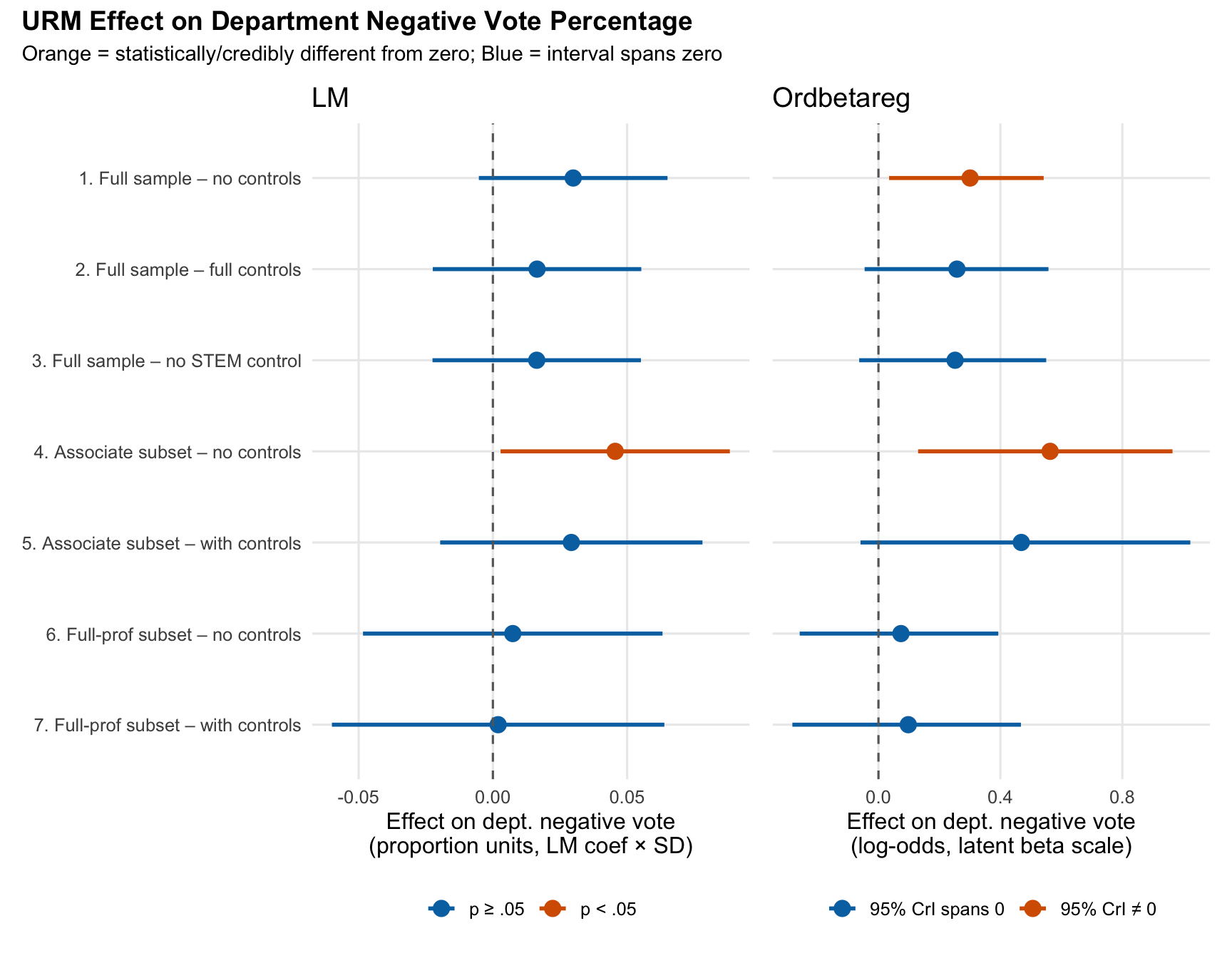
lm_plot + ord_plot +
plot_annotation(
title = "URM Effect on Department Negative Vote Percentage",
subtitle = "Orange = statistically/credibly different from zero; Blue = interval spans zero",
theme = theme(plot.title = element_text(size = 14, face = "bold"))
)