N <- 8900000

stations <- 11000

vote_assign <- sample(1:stations,N,replace=T,
                      prob=sample(1:3,stations,replace=T))

sample_size <- 1000I am writing this post in response to questions about estimating turnout for Tunisia’s constitutional referendum today. Turnout is an important aspect to this referendum because high turnout would signal higher legitimacy for President Kais Saied’s dramatic changes to the Tunisia’s democracy. His proposed constitution would replace Tunisia’s democratic institutions with a new dictatorship that would concentrate power in the president’s hands.
Because of Saied’s interference in the election commission, we are much less sure about the accuracy of results from the official election commission, the ISIE. Saied has also banned foreign election observers from arriving, leaving only one local NGO, Mourakiboun, observing polling stations. Mourakiboun has done significant work in prior elections, but reportedly faces a shortfall of local participants because of low interest in the referendum.
Mourakiboun uses a method known as parallel vote tabulation (PVT) to estimate turnout. It is a method used by NGOs like NDI to provide an independent estimate of turnout. According to NDI, to estimate turnout through observers without bias, Mourakiboun has to select a random sample of polling stations and then accurately record all votes from these polling stations. I will use some code-based simulations to see how well this method will work depending on levels of turnout. If turnout is low, there is likely to be much more sampling uncertainty because there are fewer voters at polling stations to base estimates on. I will also examine what happens if Mourakiboun does not select polling stations at random, which is likely to happen for logistical reasons. For example, Mourakiboun may put more observers at stations with higher turnout in order to save volunteer hours.
The results of the simulation show that PVT/Mourakiboun turnout estimates are probably going to be less precise at low levels of turnout compared to high levels of turnout. In addition, when turnout is low and selection of polling stations is somewhat biased, such as selecting higher-turnout polling stations, the inaccuracies in the estimates get much worse. In other words, if Mourakiboun is using an imperfect methodology and turnout is low, their estimates will be farther off than if turnout in the referendum was high. If 50% of Tunisians voted, this wouldn’t be as much of a problem, but if 10% vote, it will be much harder to get an accurate estimate using PVT via polling station counts.
Without digging into the methods below, the results can be summarized as:
If turnout is large, these biases have a much smaller role, but when turnout is small, as is likely to be the case with the constitutional referendum, the biases can have a much bigger impact on the final estimates, making Mourakiboun’s methods more likely to fail.
Simulation
First, we randomly create polling stations roughly corresponding to Tunisia’s population of 7 million registered voters and 4,500 polling stations:
What we will do is test how accurate samples will be depending on total turnout and the quality of samples. To do so, I’ll first vary true turnout from 5% up to 50% of the population. We’ll assume as well that turnout varies by polling station, which is much more accurate than assuming a constant rate of turnout for all polling stations.
We’ll assume that the stations can vary in size up to a 3-fold magnitude, i.e., some stations may be 3 times smaller than other stations. For our sample, we have a polling station as large as 1329 and one as small as 331. We’ll then assume, for now, that Mourakiboun selects a random sample of 50 polling stations and it records all votes at these stations. We’ll repeat this experiment 1,000 times and record what estimated turnout Mourakiboun would report and how that compares to real turnout:
# loop over turnout, sample polls, estimate turnout

over_turnout <- parallel::mclapply(seq(.05,.5,by=.1), function(t) {

    # polling station varying turnout rates

    station_rates <- rbeta(n=N,t*20,(1-t)*20)

    # randomly let voters decide to vote depending on true station-level turnout rate

    pop_turnout <- lapply(1:stations, function(s) {
                    tibble(turnout=rbinom(n=sum(vote_assign==s), size=1,prob =
                                            station_rates[s]),
                           station=s)
                    }) %>% bind_rows

    over_samples <- lapply(1:1000, function(i) {

        # sample 100 random polling stations 1,000 times
        sample_station <- sample(1:stations, size=sample_size)

        turn_est <- mean(pop_turnout$turnout[pop_turnout$station %in% sample_station])

        return(tibble(mean_est=turn_est,
                      experiment=i))

    }) %>% bind_rows %>%
      mutate(Turnout=t)

    over_samples

    },mc.cores=10) %>%
  bind_rows
We can now plot estimated versus actual turnout. If we have random samples and no problems with recording votes, this works fairly well. The dot shows the average of all samples, which is un-biased, and the vertical line shows where 95% of the samples fall, which is an estimate of potential sampling error. In other words, if Mourakiboun does everything right with a sample of 50 polling stations, they would expect this kind of error from random chance alone. If true turnout is 15%, they could see estimates that range from 12% to 17%.
over_turnout %>%
  group_by(Turnout) %>%
  summarize(pop_est=mean(mean_est),
            low_est=quantile(mean_est,.05),
            high_est=quantile(mean_est, .95)) %>%
  ggplot(aes(y=pop_est,x=Turnout)) +
  geom_pointrange(aes(ymin=low_est,
                      ymax=high_est),size=.5,fatten=1) +
  geom_abline(slope=1,intercept=0,linetype=2,colour="red") +
  theme_tufte() +
  theme(text=element_text(family="")) +
  labs(y="Estimated Turnout",x="True Turnout",
       caption=stringr::str_wrap("Comparison of Mourakiboun estimated (y axis) versus actual turnout (x axis). Red line shows where true and estimated values are equal. Based on random samples of 50 polling stations and assuming no problems with recording votes."))
Unfortunately, this kind of accuracy only happens in a computer simulation. It is quite tricky to do a true random sample of polling stations because there may not be volunteers to cover all of the polling stations, as is the case with the current referendum. Let’s assume in the following simulation then that a polling station is more likely to be sampled if the true level of turnout is higher:
# loop over turnout, sample polls, estimate turnout

over_turnout_biased <- parallel::mclapply(seq(.05,.5,by=.1), function(t) {

    # polling station varying turnout rates

    station_rates <- rbeta(n=stations,t*20,(1-t)*20)

    # randomly let voters decide to vote depending on true station-level turnout rate

    pop_turnout <- lapply(1:stations, function(s) {
                    tibble(turnout=rbinom(n=sum(vote_assign==s), size=1,prob =
                                            station_rates[s]),
                           station=s)
                    }) %>% bind_rows

    over_samples <- lapply(1:1000, function(i) {

        # sample 100 random polling stations 1,000 times
        sample_station <- sample(1:stations, size=50,prob=station_rates)

        turn_est <- mean(pop_turnout$turnout[pop_turnout$station %in% sample_station])

        return(tibble(mean_est=turn_est,
                      experiment=i))

    }) %>% bind_rows %>%
      mutate(Turnout=t)

    over_samples

    },mc.cores=10) %>%
  bind_rows
We can now plot estimated versus actual turnout for this simulation where the polling stations were more likely to be sampled if they had higher turnout:
over_turnout_biased %>%
  group_by(Turnout) %>%
  summarize(pop_est=mean(mean_est),
            low_est=quantile(mean_est,.05),
            high_est=quantile(mean_est, .95)) %>%
  ggplot(aes(y=pop_est,x=Turnout)) +
  geom_pointrange(aes(ymin=low_est,
                      ymax=high_est),size=.5,fatten=1) +
  geom_abline(slope=1,intercept=0,linetype=2,colour="red") +
  theme_tufte() +
  theme(text=element_text(family="")) +
  labs(y="Estimated Turnout",x="True Turnout",
       caption=stringr::str_wrap("Comparison of Mourakiboun estimated (y axis) versus actual turnout (x axis). Red line shows where true and estimated values are equal. Based on biased samples of 50 polling stations with higher turnout stations more likely to be sampled. However, simulation assumes no problems with recording votes.")) +
  ylim(c(0,0.5)) +
  xlim(c(0,0.5))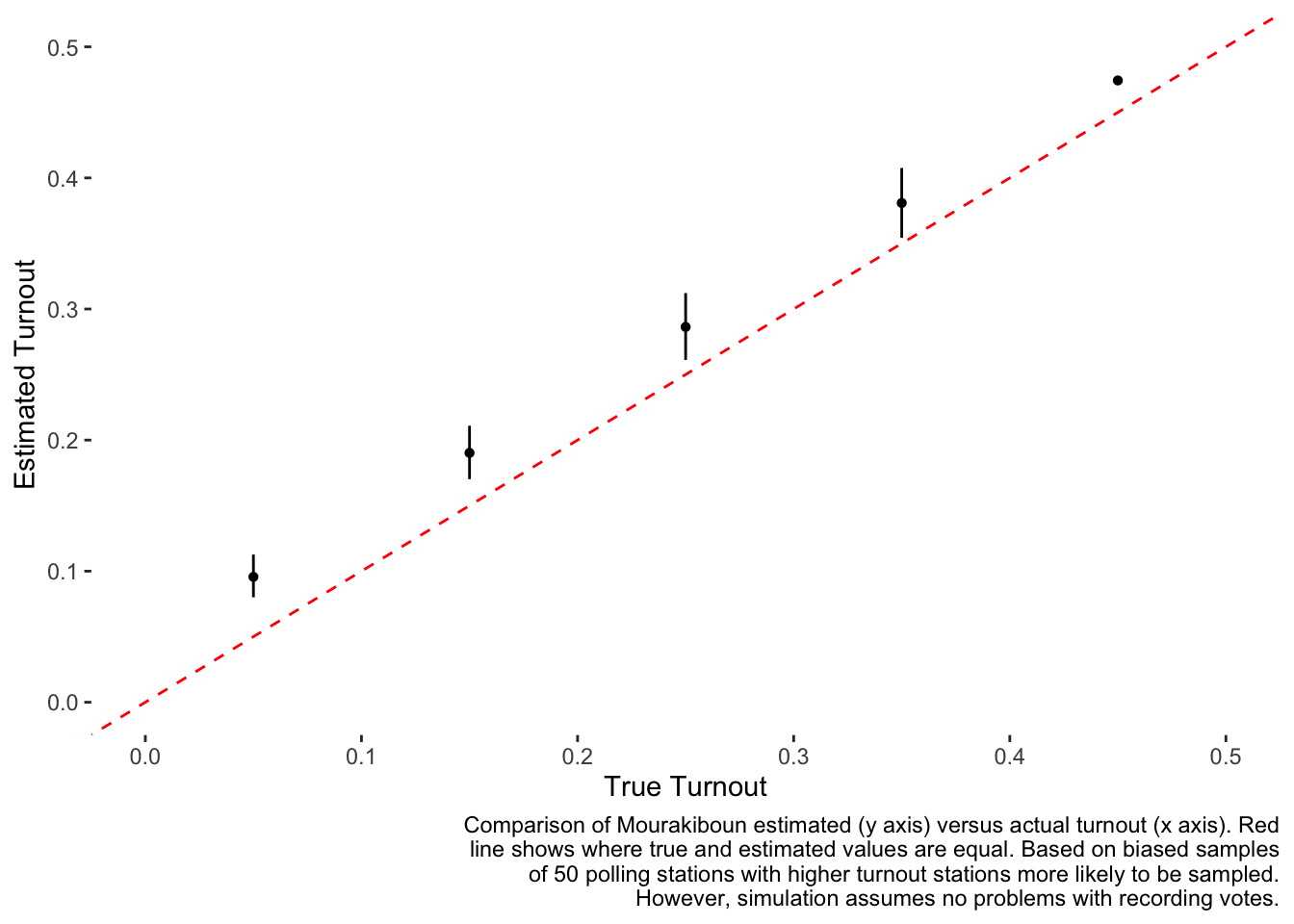
We see in the plot above that the black dot estimates are always higher than the red line showing the true values. Furthermore, the bias appears worse when turnout is smaller. The bias is also substantial - at low levels of turnout, such as at 5%, the estimated turnout can be twice as high.
As can be seen in this simulation study, it is quite possible for the method to work, but only if the polling stations are selected at random. I did not look into what would happen with other possible errors, such as being unable to accurately record all votes from a given polling station. For these reasons, while this method can certainly work, it is necessary to confirm what methodology was used to select the polling stations and also how strictly it was followed in implementation. There are many points at which this type of analysis could either intentionally or unintentionally result in over/under reporting of turnout.
If turnout is large, some of these biases have a minimal effect, but when turnout is small, as is likely to be the case with the constitutional referendum, they can have a much bigger impact on the final estimates.