# use the mean/variance parameterization of the beta distribution

pt <- 393/151268
pc <- 655/75634

# Generate values for VE given beta distributions for pt/pc

VE <-  1 - rbeta(10000,pt*5000,(1-pt)*5000)/rbeta(10000,pc*5000,(1-pc)*5000)

hist(VE)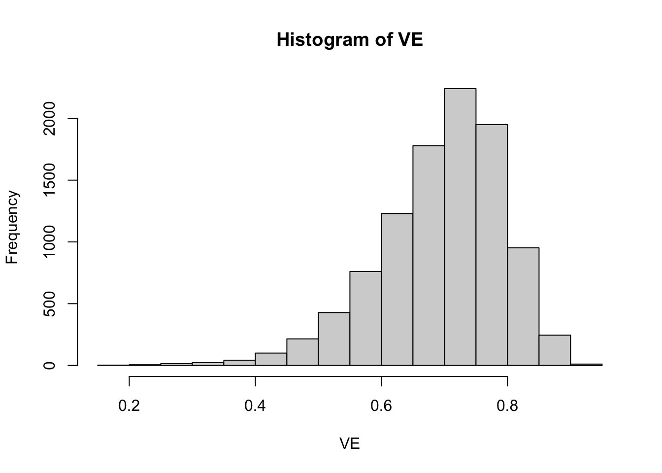
Read my latest on 5 lessons from political science to help rebuild Syria in The Conversation.
In this blog post, I use Gelman and Loken’s garden of forking paths analysis to construct a simulation showing why skepticism of AstraZeneca’s vaccine results is warranted at this early stage. This simulation uses the numbers from their press release to illustrate how noise in treatment regimes can undermine serendipitous results. As Gelman and Loken describe, researchers can stumble on conclusions which they are then very able to provide post hoc justifications for. Unfortunately, when incentives to get results are strong, human beings are also very likely to focus on the positive at the expense of obtaining the full picture.
Similar to my last post on Pfizer’s vaccine, I start with Eric Novik’s excellent blog post on how to calculate the relevant statistics for the vaccine, i.e. vaccine efficacy (VE). This is defined as:
Where
They don’t give us all the information to figure out how many people were infected with COVID-19 in treatment versus control, but we can infer
Thankfully, this system has a single solution where
# use the mean/variance parameterization of the beta distribution
pt <- 393/151268
pc <- 655/75634
# Generate values for VE given beta distributions for pt/pc
VE <- 1 - rbeta(10000,pt*5000,(1-pt)*5000)/rbeta(10000,pc*5000,(1-pc)*5000)
hist(VE)
This plot shows that the true VE in the population is on average 0.7 but could vary substantially. It could be below 0.5 for a small subset of the population and above 0.9 for a small subset of the population. To simulate our data, we will draw VEs from this beta distribution separately for each of four possible subgroups
Four subgroups are chosen to be roughly equal to the size of the half-dose group in the AstraZeneca study given a sample size of 11,636. I add a further step in that I assume that the probability of VE being reported for a subgroup
This equation shows that the extent of the bias in using only reported results is equal to
The R code to generate this model in terms of treatment/control COVID cases and whether or not subgroup analyses are reported is as follows:
# number of samples

N <- 1000

sim_data <- lapply(1:N,function(n) {

  # generate subgroup treatment/control COVID proportions

  sub_pt <- rbeta(4,pt*5000,(1-pt)*5000)
  sub_pc <- rbeta(4,pc*5000,(1-pc)*5000)


  # generate subgroup VEs

  VE <-  1 - sub_pt/sub_pc

  # generate COVID case data with binomial distribution

  covid_t <- sapply(sub_pt, function(pt) rbinom(n=1,size = floor(11636/4),prob=pt))
  covid_c <- sapply(sub_pc, function(pc) rbinom(n=1,size = floor(11636/4),prob=pc))

  # output data

  tibble(draw=n,
         groups=1:4,
         sub_pt=sub_pt,
         sub_pc=sub_pc,
         VE=VE,
         VE_r=as.numeric(runif(n=4)<plogis(-250 + 300*VE)),
         covid_t = covid_t,
         covid_c=covid_c)

}) %>% bind_rows
Given this simulation, only a minority (4%) of subgroup analyses are reported. The average VE for the reported subgroups is 77% as opposed to a VE of 69% across all simulations. As such, the simulation assumes that it is unlikely that subgroups with low vaccine efficacy will end up being reported, while subgroups with stronger efficacy are more likely to be reported.
For each random draw from the simulation, I can then fit a model that analyses only those analyses that are reported:
# modified code from Eric Novik

vac_model <- "data {
  int g; // number of sub-groups
  array[g] int<lower=0> r_c; // num events, control
  array[g] int<lower=0> r_t; // num events, treatment
  array[g] int<lower=1> n_c; // num cases, control
  array[g] int<lower=1> n_t; // num cases, treatment
}
parameters {
  array[g] real<lower=0, upper=1> p_c; // binomial p for control
  array[g] real<lower=0, upper=1> p_t; // binomial p for treatment
}
transformed parameters {
  real VE = mean(1 - to_vector(p_t) ./ to_vector(p_c));  // average vaccine effectiveness across groups
}
model {
  p_t ~ beta(2, 2); // weakly informative,
  p_c ~ beta(2, 2); // centered around no effect
  r_c ~ binomial(n_c, p_c); // likelihood for control
  r_t ~ binomial(n_t, p_t); // likelihood for treatment
}
generated quantities {
  vector[g] effect   = to_vector(p_t) - to_vector(p_c);      // treatment effect
  vector[g] log_odds = log(to_vector(p_t) ./ (1 - to_vector(p_t))) -
                           log(to_vector(p_c) ./ (1 - to_vector(p_c)));
}"

to_stan <- cmdstan_model(write_stan_file(vac_model))


est_bias <- lapply(unique(sim_data$draw), function(i) {

  sink("output.txt")

  this_data <- filter(sim_data,draw==i,VE_r==1)

  stan_data <- list(g=length(unique(this_data$groups)),
                    r_c=as.array(this_data$covid_c),
                    r_t=as.array(this_data$covid_t),
                  n_c=as.array(round(rep(floor(11636/4),
                                length(unique(this_data$groups)))/2)),
                  n_t=as.array(round(rep(floor(11636/4),
                                length(unique(this_data$groups)))/2)))

  if(stan_data$g<1) {
    tibble(draw=i,
           VE=NA)

  } else {
    est_mod <- to_stan$sample(data=stan_data,
                              seed=624018,
                              chains=1,iter_warmup=500,iter_sampling=1000,refresh=500)

    draws <- est_mod$draws() %>% as_draws_df

    tibble(draw=i,
         VE=draws$VE)
  }

  sink()

}) %>% bind_rows
I can then plot the density of the estimated reported VE from this simulation along with a line indicating the true average VE in the population:
est_bias %>%
  ggplot(aes(x=VE)) +
  geom_density(fill="blue",alpha=0.5) +
  geom_vline(xintercept=mean(sim_data$VE),linetype=2) +
  theme_tufte() +
  xlim(c(0,1)) +
  xlab("Reported VE") +
  ylab("") +
  annotate("text",x=mean(sim_data$VE),y=3,label=paste0("True VE = ",round(mean(sim_data$VE)*100,1),"%"))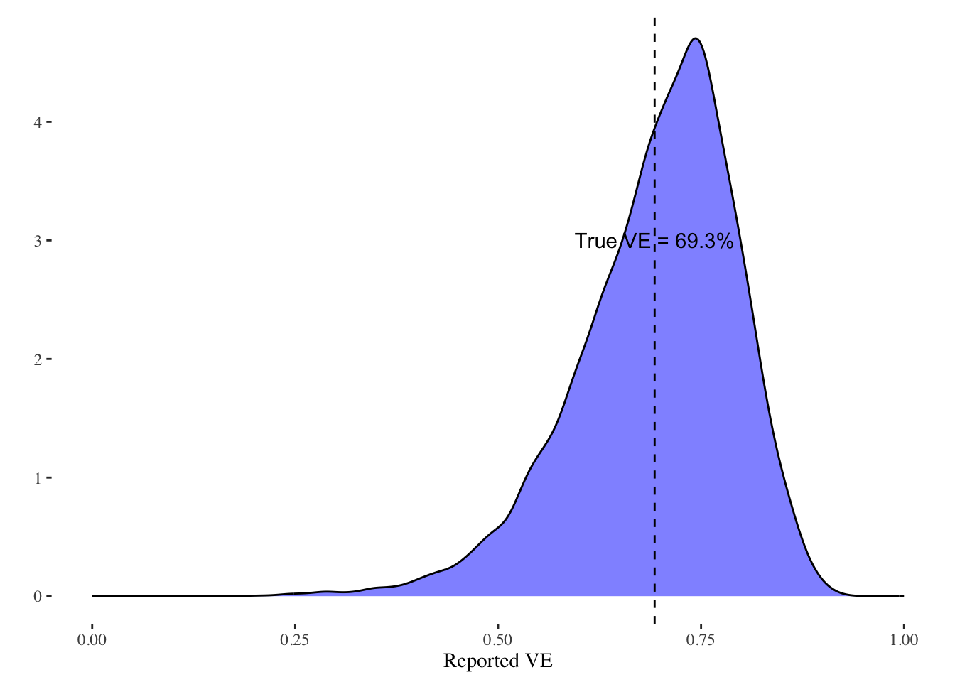
As can be seen, it is much more likely that VEs higher than the true average VE will be reported. The extent of the bias is driven by the simulation and how much weight the simulation puts on discovering high VE values. Given the profit that AstraZeneca stands to gain, and the fame and prestige for the involved academics, it would seem logical that reported analyses from subgroups will tend to be subgroups that out-perform the average.
Note that this simulation shows how AstraZeneca could be reporting valid statistical results, yet these results can still be a biased estimate of what we want to know, which is how the vaccine works for the population as a whole. The possibility of random noise in subgroups and the fact that subgroups are likely to respond differently means that we should be skeptical of analyses that only report certain subgroups instead of all subgroups. Only when we understand the variability in subgroups can we say whether the reported finding in AstraZeneca’s press release represents a real break-through or simply luck. Of course, they can test it directly by doing another trial, which it seems to be is their intention. Serendipity, though, isn’t enough of a reason to trust these results unless we can examine all of their data.